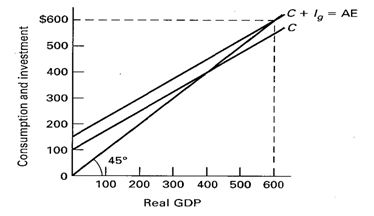
Use the graph below to explain the determination of equilibrium GDP by the aggregate expenditures-domestic output approach. At equilibrium C + Ig = Real GDP ($550 + $50 = $600). Why does the intersection of the aggregate expenditures schedule and the 45-degree line determine the equilibrium GDP?

Equilibrium occurs where C + Ig = GDP. There is a direct relationship between aggregate expenditures and the level of GDP, but they are equal only where the AE schedule intersects the 45-degree line which shows equality of expenditures and GDP. Where aggregate expenditures exceed GDP, the AE line is above the 45-degree line and output will continue to expand. If aggregate expenditures fall below GDP as would occur at levels above 600, then GDP will contract until the expenditures-output equality is restored.
The 45-degree line in the aggregate expenditures model represents all of the points where aggregate expenditures are equal to real GDP; all of the possible equilibrium levels.