Suppose that the current price of oil is $60 per barrel and the quantity sold is 90 million barrels per day
The current estimates of the price elasticity of supply and demand are ? = 1 and
? = -.2 respectively. What will be the effects on the market price and quantity if the U.S. government suddenly decides to purchase an additional 2 million barrels of oil? Assume that the supply and demand curves are linear and the addition consumption of oil by the government results in a parallel shift of the supply curve to the left by 2 million barrels per day.
First use the elasticities and current price and quantity to estimate the linear demand and supply equations:
1 = (slope of supply) × (60 per barrel)/(90 million)
Thus the slope of the supply curve is 1.5. Using the current price and quantity, we can solve for the supply curve intercept:
QS = A + 1.5p
90 = A + 1.5 (60)
A = 0
The supply curve is then given by QS = 1.5p. Repeat this process to find the demand equation:
-.2 = (slope of demand) × (60 per barrel)/(90 million)
The slope of the demand curve is -.3. The intercept is 108 so the demand equation is :
QD = 108-0.3p
The supply curve following the government's purchase of oil will become:
QS = 1.5p - 2
Setting supply and demand equal to find equilibrium price:
1.5p - 2 = 108 - .3p
p = 61.11
The quantity if found from plugging the price into either the (new) supply or demand equation. barrels per day. Thus the purchase of oil by the government increases the price and reduces the quantity sold in the market. Including the government's purchase of 2 million barrels, the quantity increases to 91.67. Thus the government purchase crowded out .33 million barrels of private consumption of oil.
You might also like to view...
How does total taxes as a percentage of GDP in the United States compare to those of Western European countries, such as the United Kingdom, Germany, and Sweden?
a. U.S. taxation is smaller. b. U.S. taxation is about the same. c. U.S. taxation is slightly larger. d. U.S. taxation is substantially larger.
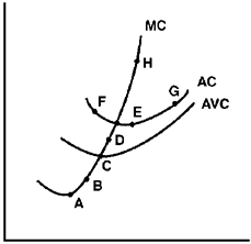
Figure 10-5

In Figure 10-5, points which lie on the firm's short-run supply curve are
a.
A, B, C.
b.
C, D, H.
c.
F, E, G.
d.
A, C, H.